Overview
There is a closed-form solution to phased array beam steering. Given N antenna elements and a target direction θ₀, the optimal per-element phase offsets are ψₙ = -k·n·d·sin(θ₀), derivable in a few lines from the wave equation. So why implement a gradient ascent optimizer?
Because the closed form only exists for the simple case. Extend the problem to adaptive interference nulling, where you must simultaneously steer toward a target and carve a null in a jammer's direction, and no equivalent formula falls out. The optimizer generalizes; the analytical solution does not.
This project builds a complete phased array simulator in MATLAB from first principles: 1D linear arrays, 2D planar arrays, and a fully derived gradient ascent optimizer that independently recovers the analytical solution in both cases. That agreement is the actual validation. Adaptive nulling via a SINR objective is the planned next step.
Wave Physics Foundation
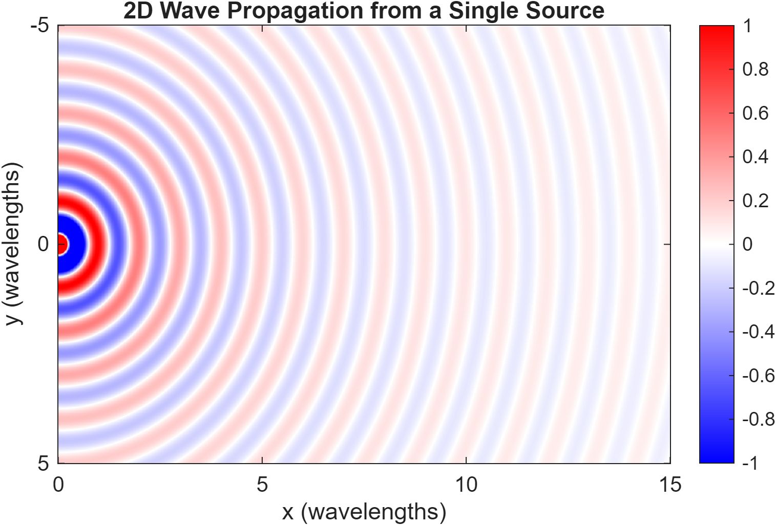
The field radiated by a single isotropic point source at (x₀, y₀) is modeled as a spherical wave:
E(X, Y) = (E₀ / R) · exp(-j·k·R)where R is source-to-field-point distance and k = 2π/λ is the wavenumber. Adding eps to R before division resolves the 1/R singularity at the source cleanly, with no conditional logic and negligible effect beyond a fraction of a wavelength.
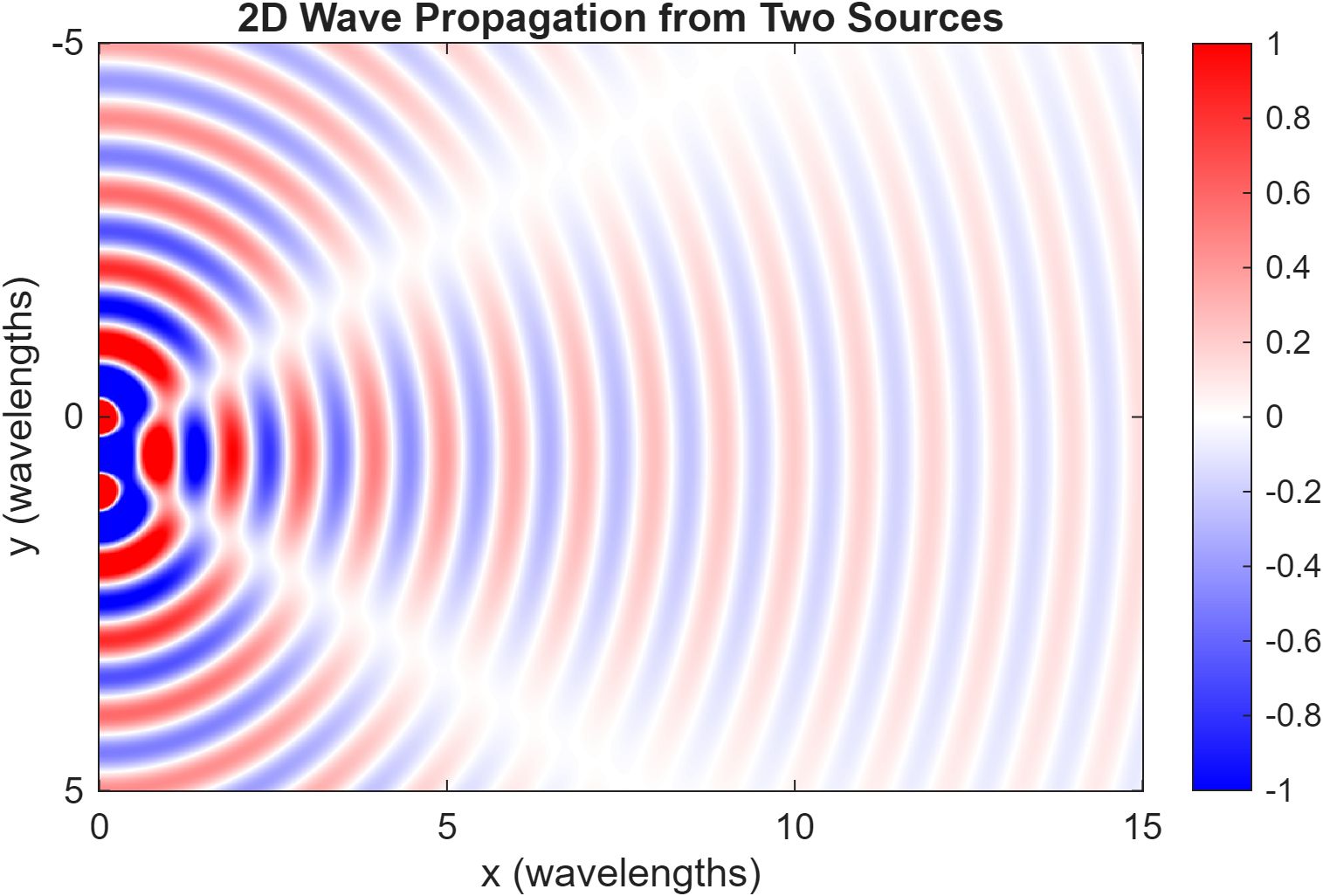
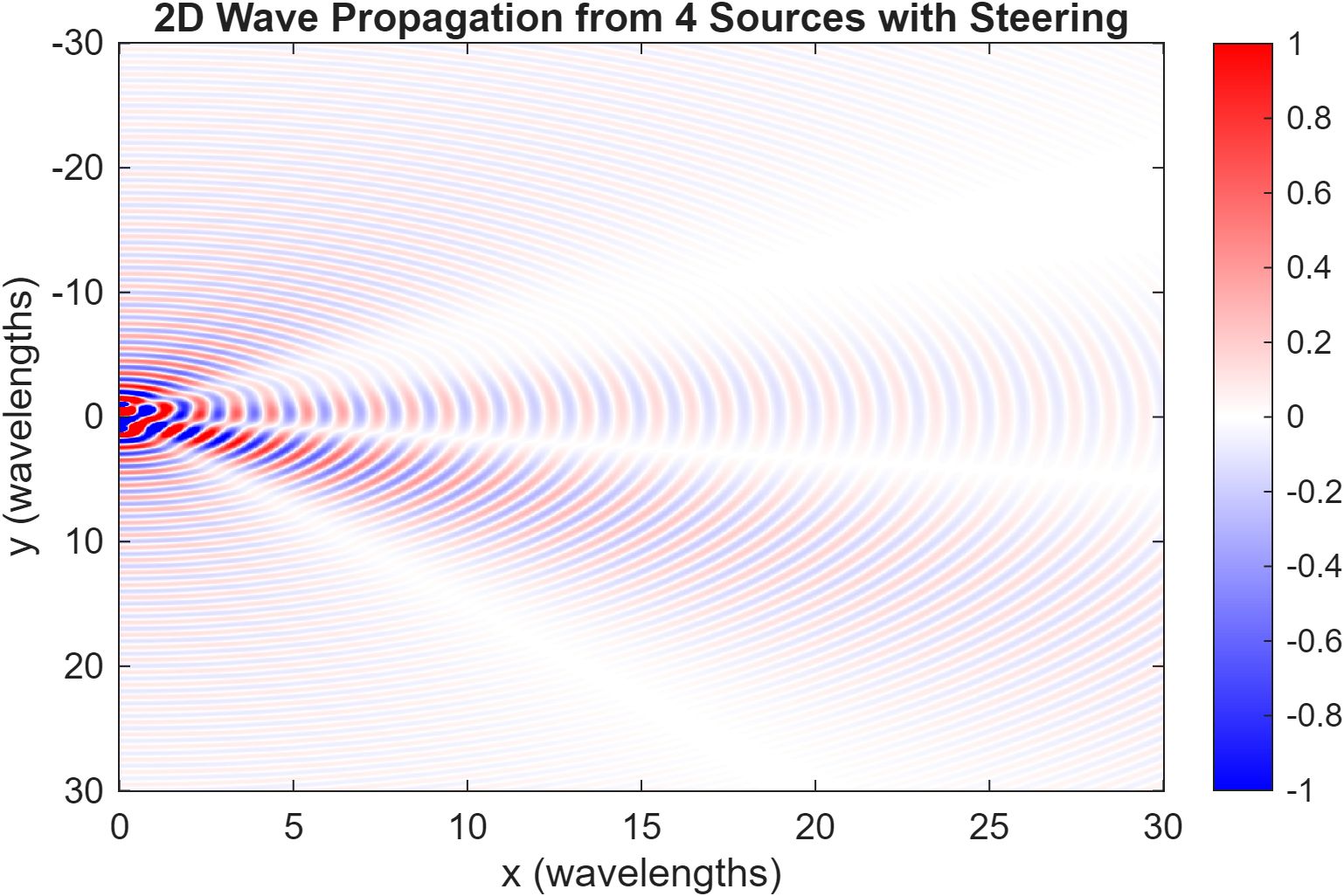
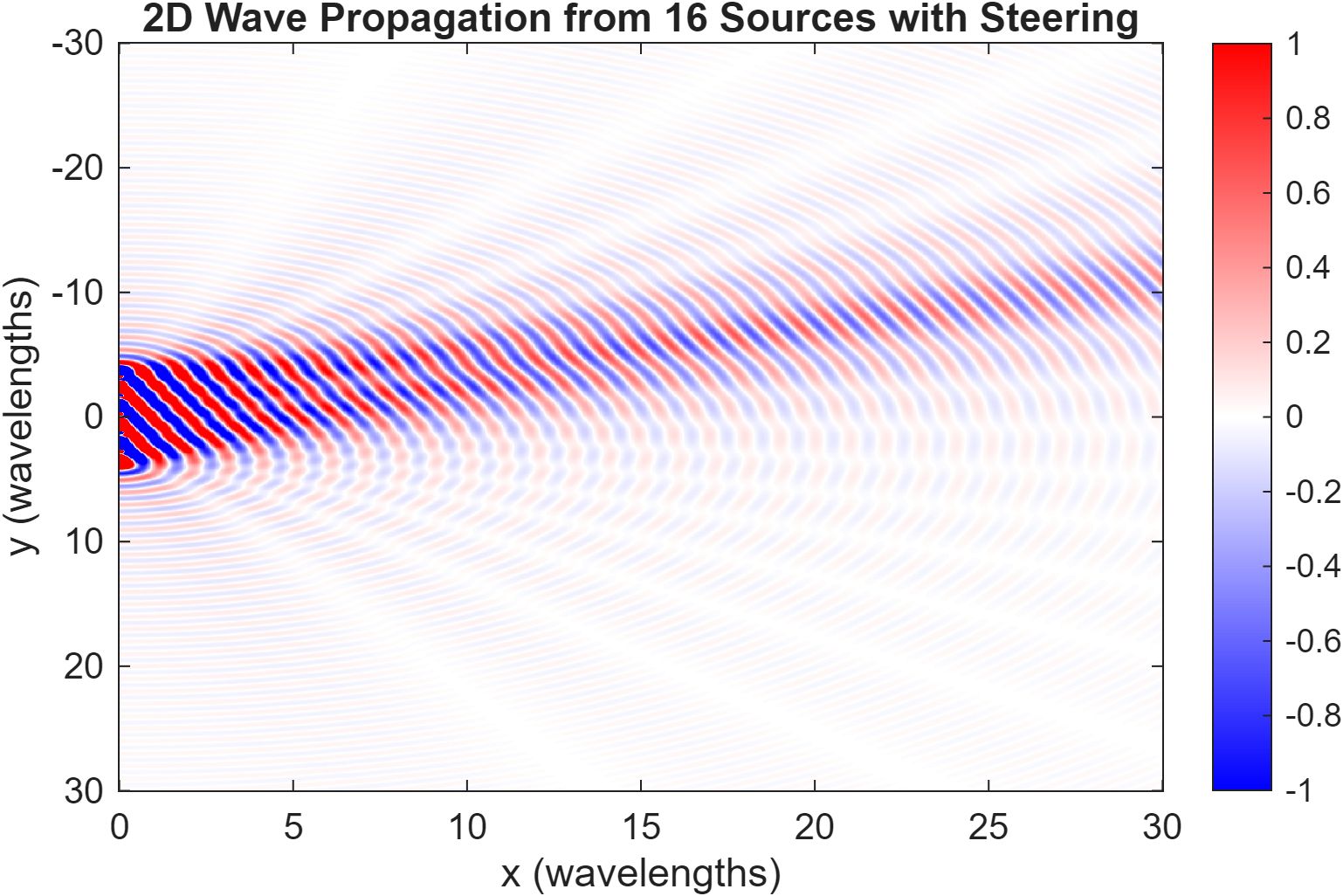
Superposing the fields from all array elements, each weighted by its phase offset ψₙ, produces the interference patterns that make beamforming work.
Array Factor and Beam Steering
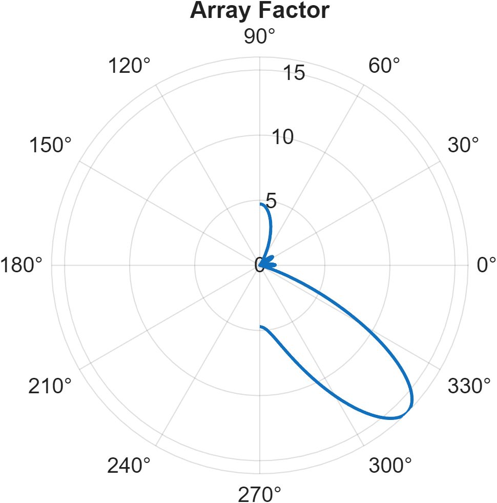
For a linear array of N elements spaced d = λ/2 along the y-axis, the path length from element n to a far-field observation point at angle θ exceeds element 0's path by n·d·sin(θ). This introduces a geometric phase advance of k·n·d·sin(θ). Summing all element contributions gives the Array Factor:
AF(θ) = Σ exp(j·(k·d·n·sin(θ) + ψₙ))The radiated power pattern is |AF(θ)|². The closed-form steering solution follows directly: to make all N contributions arrive in phase at θ₀, each element's phase offset cancels its geometric delay:
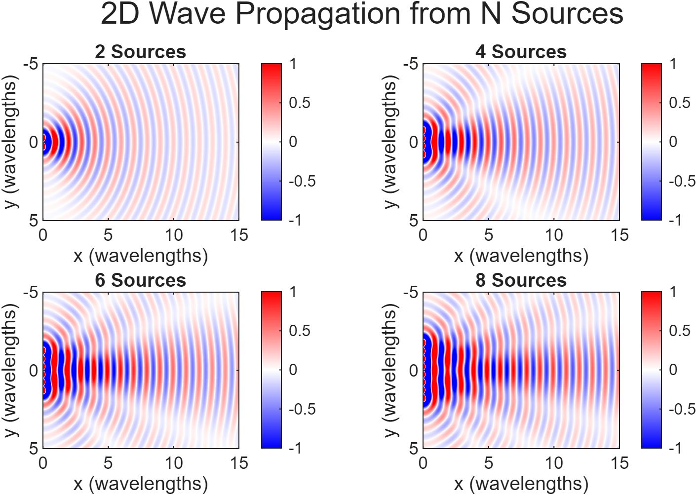
ψₙ = -k·n·d·sin(θ₀)As N increases, the main lobe narrows and side lobes shrink. More elements means a more directional antenna.
2D Planar Array Extension
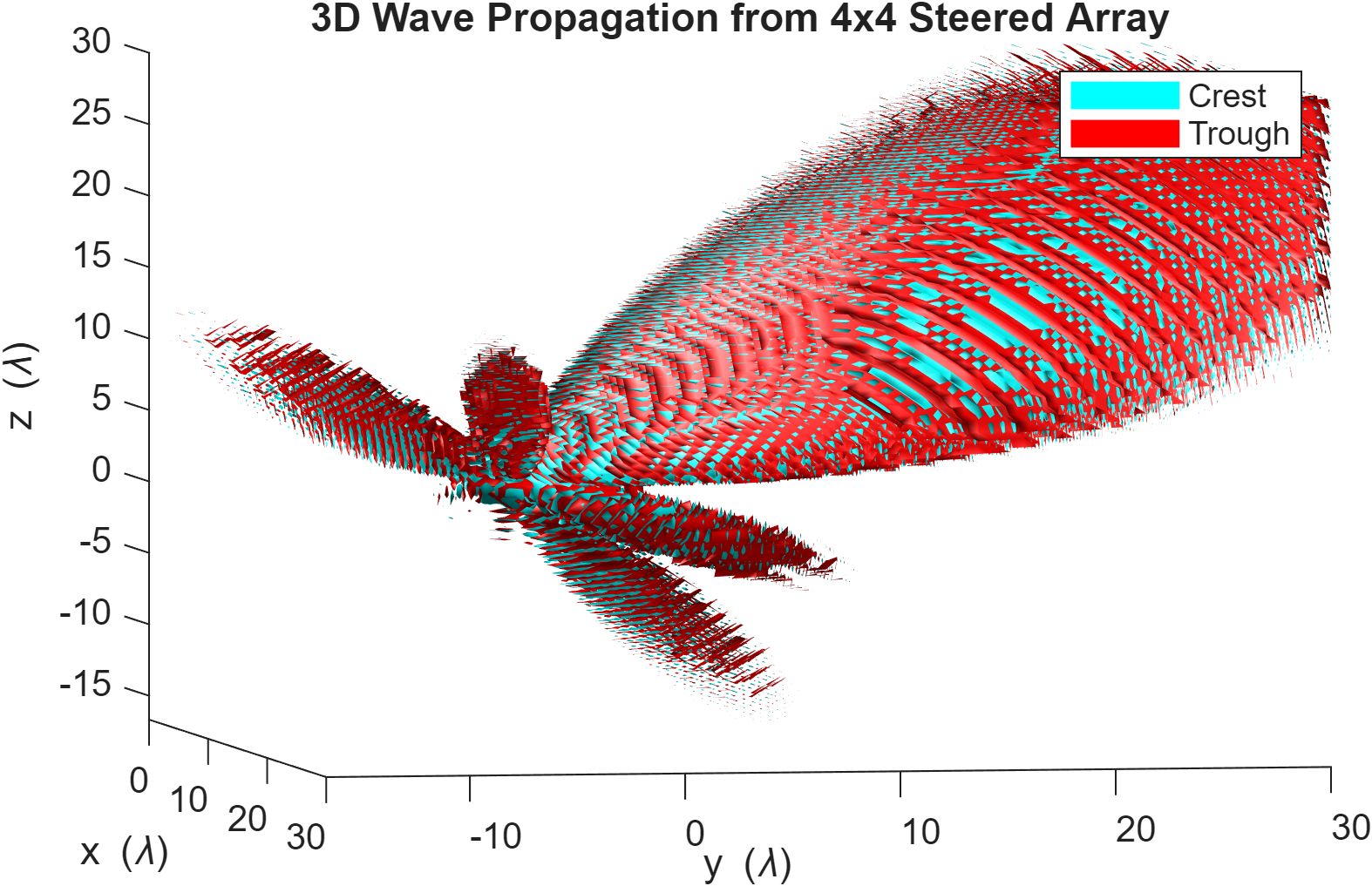
The 1D setup extends to an Ny x Nz planar array on the yz-plane. Each element at (yₘ, zₙ) now contributes two geometric phase terms:
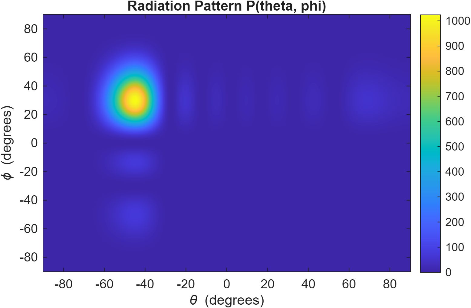
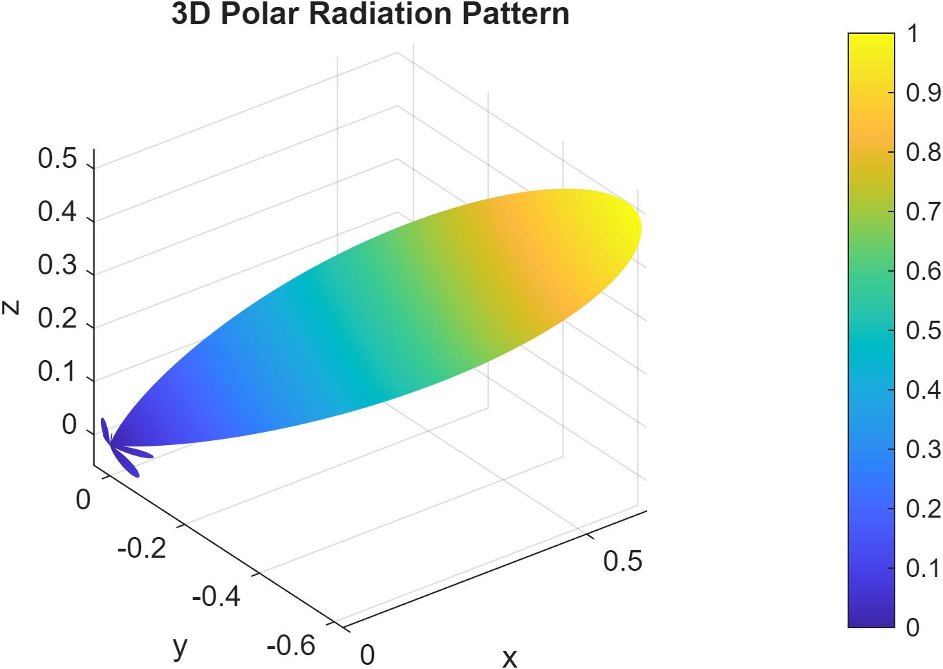
φ_geo(y, z, θ, φ) = k·y·sin(θ) + k·z·sin(φ)The array factor becomes a double sum over the full element grid, the radiation pattern P(θ, φ) lives on a 2D angular grid, and total power requires nested integration over both dimensions. Analytical steering generalizes to:
ψₙ = -k·(yₙ·sin(θ₀) + zₙ·sin(φ₀))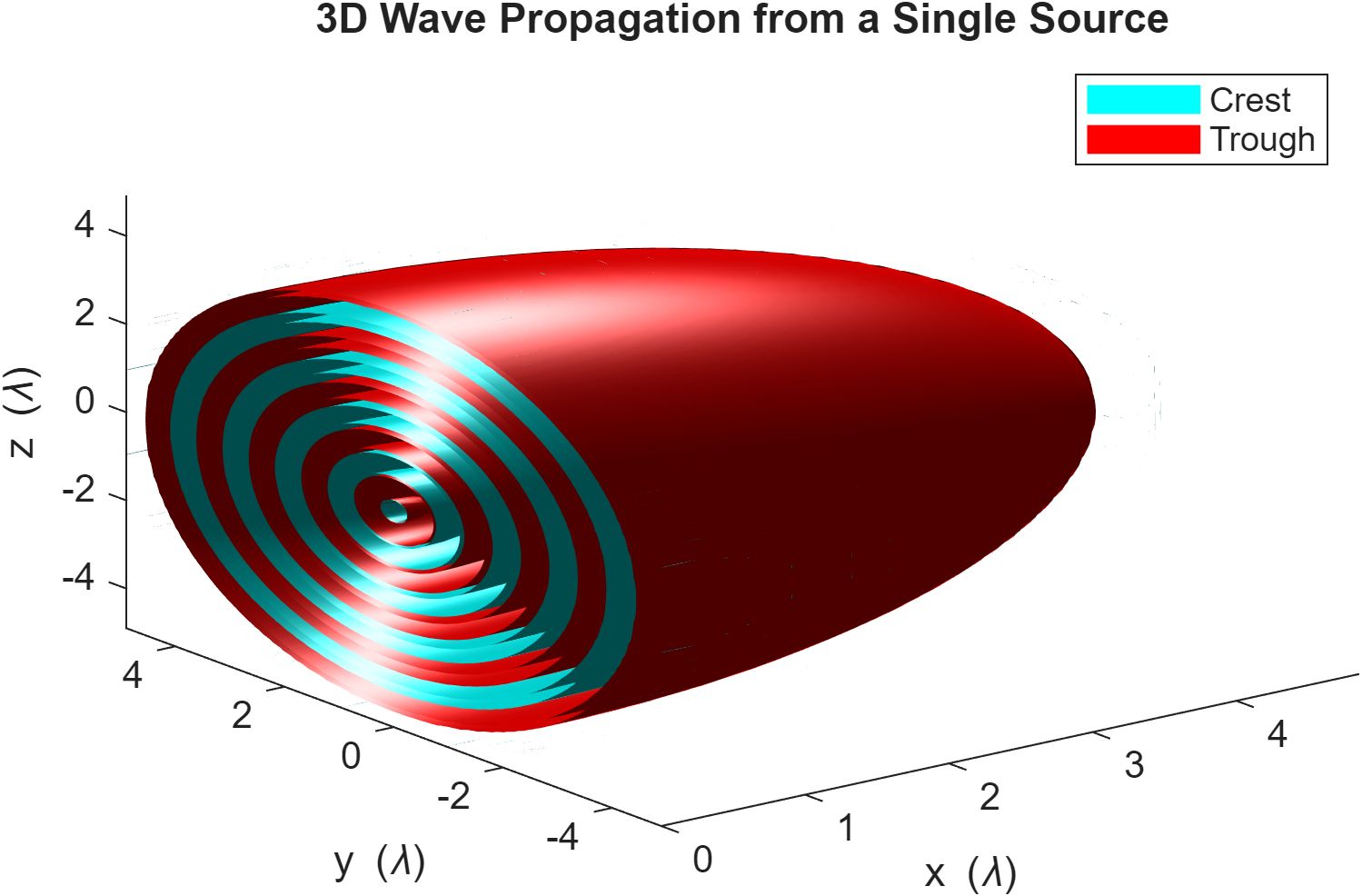
Gradient Ascent Optimizer
The analytical solution is elegant but limited to the simple case. The optimizer treats ψ as a free variable and maximizes a gain objective directly, which is the approach that generalizes to problems with no closed form.
Objective Function
The gain G(ψ) is the fraction of total radiated power concentrated at the target direction:
G(ψ) = |AF(θ₀; ψ)|² / P_total(ψ)P_total is the total power radiated across all angles, computed by numerical integration over θ ∈ [-π/2, π/2] using trapz at each iteration. Thinking about P_total geometrically: it is the area under the |AF(θ)|² curve. The cumulative integral shows where that area accumulates: most of it piles up near the main lobe, with the side lobes contributing the remainder.
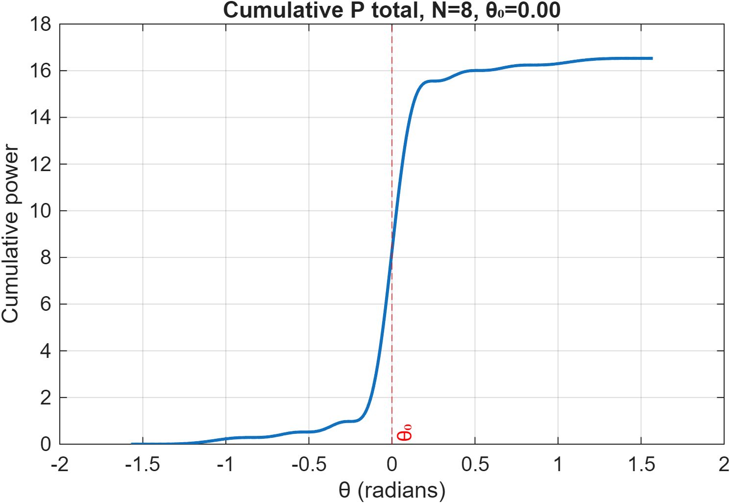
G is a scalar function of the N-dimensional phase vector ψ. It is bounded between 0 (power spread uniformly) and N (all power concentrated at the target), so gradient ascent has a finite, well-defined maximum to climb toward.
The Gradient
The key advantage of this formulation is that ∇_ψ G is available in closed form. Differentiating via the quotient rule and pulling the derivative through the integral for the P_total term gives:
dG/dψₙ = [2·Re(j·AF₀*·cₙ(θ₀))·P_total - |AF₀|²·dP_total/dψₙ] / P_total²where cₙ(θ) = exp(j·(k·n·d·sin(θ) + ψₙ)) is element n's phasor contribution at angle θ, and:
dP_total/dψₙ = ∫ 2·Re(j·AF(θ)*·cₙ(θ)) dθNo finite differences needed. The gradient is exact and cheap to evaluate given the AF values already computed for G. For the 2D array, the same structure extends to a double integral over (θ, φ), with geometric phases precomputed once as a 3D tensor before the loop so that all per-element operations inside each iteration are vectorized.
The Update Rule
Each iteration moves ψ in the direction of steepest ascent:
ψ ← ψ + α · ∇_ψ GThe step size α = 0.01 is fixed throughout. The gain landscape is smooth and convex near the optimum, so fixed α converges reliably. One implementation detail: initializing ψ = 0 places the optimizer on a symmetric saddle point where the gradient is identically zero, so ψ is initialized with small random noise to break the symmetry. The loop terminates when ‖∇G‖ < 10⁻⁴, which detects when all N phase offsets have simultaneously plateaued. This is more robust than checking individual components or the change in G, which is susceptible to plateau false positives.
Results on the 8x5 Array
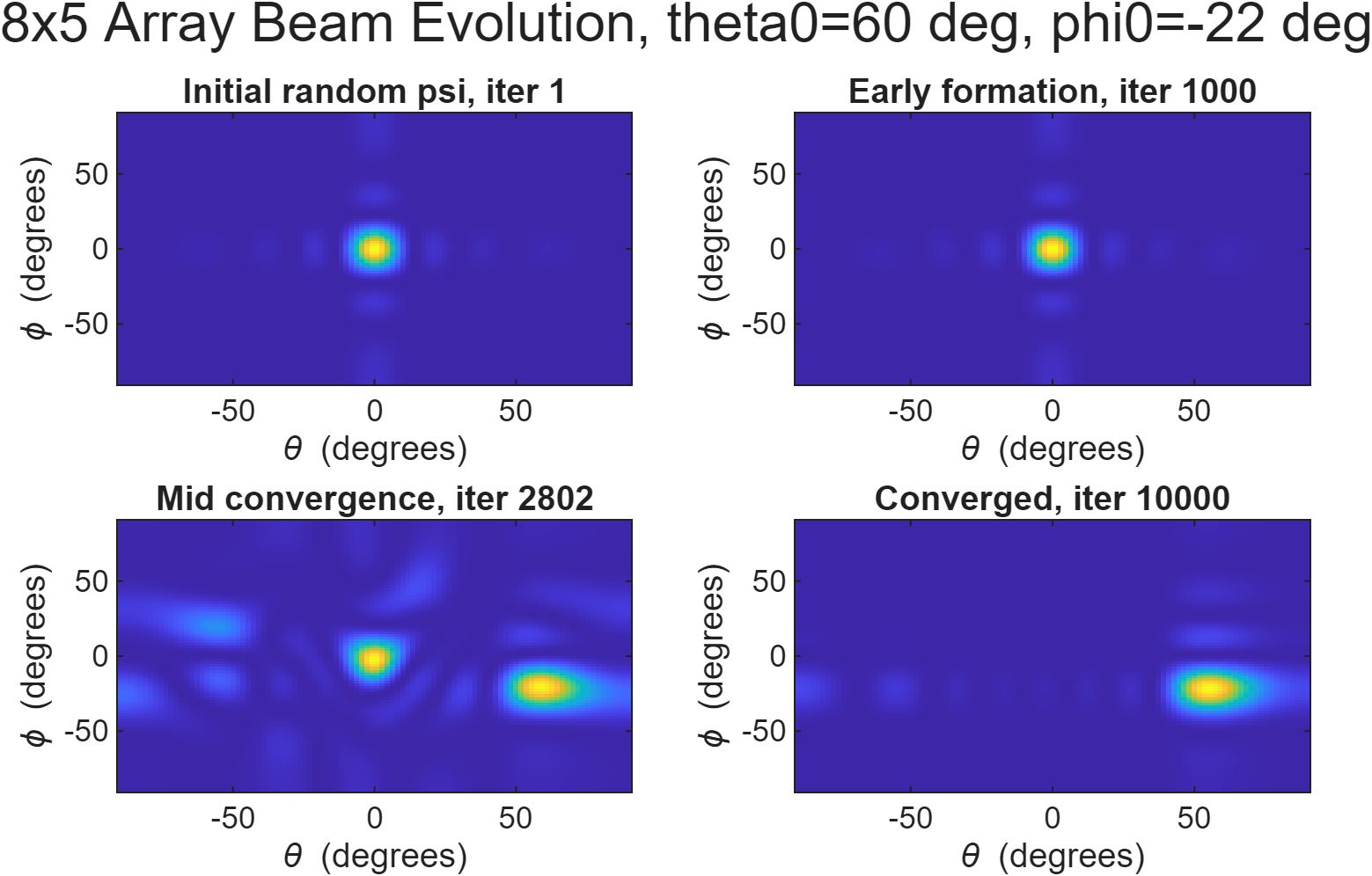
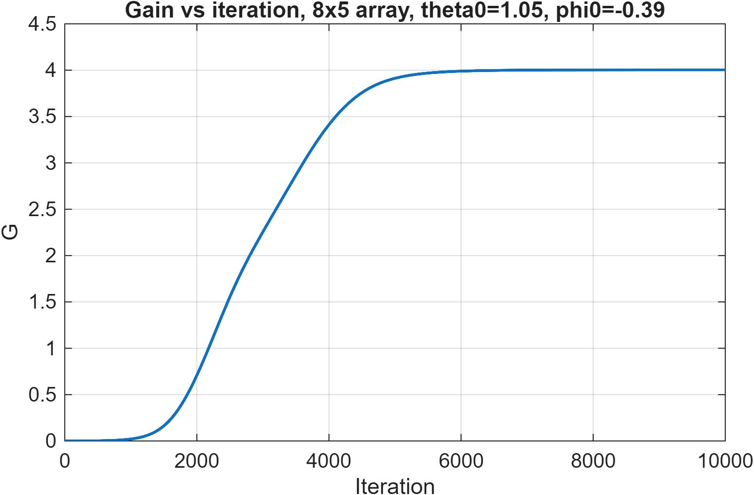
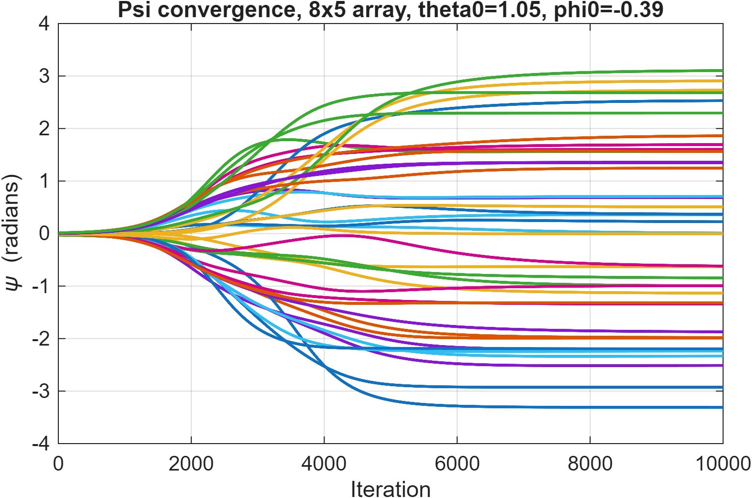
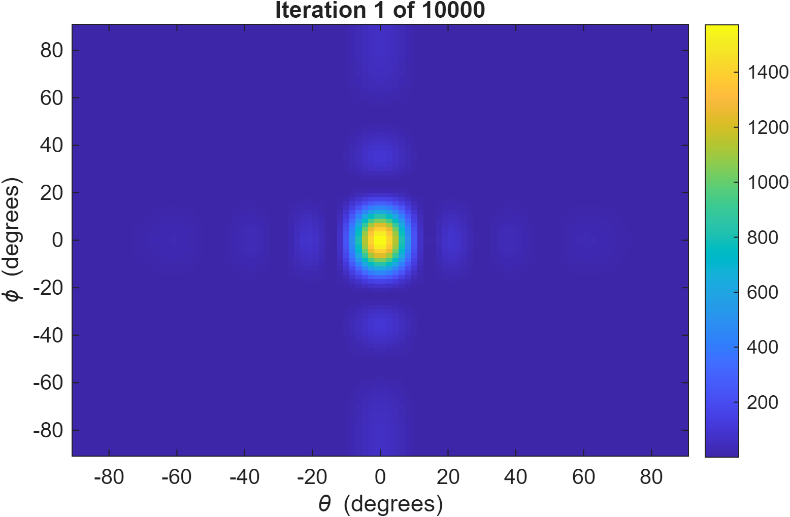
For the 8x5 array, gradient ascent converges in roughly 1000 to 3000 iterations and recovers the 2D analytical steering solution to numerical precision.
Results
| Setup | Convergence | Outcome |
|---|---|---|
| 1D, N=8 elements | ~500-1500 iterations | ψ* matches -k·n·d·sin(θ₀) to numerical precision |
| 2D, 8x5 array | ~1000-3000 iterations | ψ* matches 2D analytical solution to numerical precision |
The optimizer recovering the closed-form solution independently is the actual validation. It confirms the gradient derivation is correct, not just that the output looks plausible.
Key Engineering Insights
Validating the optimizer requires a ground truth. A visually reasonable beam could come from a buggy gradient. Numerical agreement with the known analytical solution is what makes the result trustworthy rather than merely plausible.
Symmetry breaks gradient optimizers silently. The zero-initialization failure does not throw an error or produce a visibly wrong output. It produces an immediate, confident false convergence. Recognizing saddle points as a structural property of the problem, rather than a bug to step through, is what fixed it.
The gain objective encodes the right tradeoff. Maximizing |AF(θ₀)|² alone would just scale up all phases uniformly. Dividing by P_total forces the optimizer to concentrate power, not just increase it. The normalization is what makes G a meaningful objective for beamforming.
Next Steps
The gradient ascent formulation is more general than the closed-form solution, which is the whole point of building it. The natural next target is adaptive interference nulling: simultaneously maximize gain toward a target while suppressing a jammer.
This means replacing G(ψ) with a Signal-to-Interference-plus-Noise Ratio (SINR) objective:
G_SINR(ψ) = |AF(θ₀, φ₀)|² / (|AF(θ_j, φ_j)|² + ε·P_total)The denominator penalizes power in the jammer direction (θ_j, φ_j). The ε·P_total term prevents the degenerate solution where the optimizer collapses all radiation to zero, which would achieve infinite SINR trivially via 0/0. The ε parameter controls the tradeoff between null depth and main lobe gain. The SINR gradient follows the same quotient rule structure as the current gain gradient, so no changes to the optimizer loop are needed.
The null is not placed explicitly. It emerges from the objective, the same way the main lobe emerges from maximizing G. That is what makes this formulation interesting: it is the same math used in 5G massive MIMO beamforming and radar electronic protection, just at a scale where the structure is legible.